Since we are all about advantages (and disadvantages) of LLMs, we quickly overlook how difficult it is for machines to assist us outside the virtual chat interfaces. People are getting older, work and professions are changing, but we still need to fold our clothes and sort our dishes at the end of the day, for a lot of days to come. The feeling lingers that the physical breakthrough for AI is just around the corner, ready to literally knock our front door down and aggressively scrub our toilets.
| Gif |
|---|
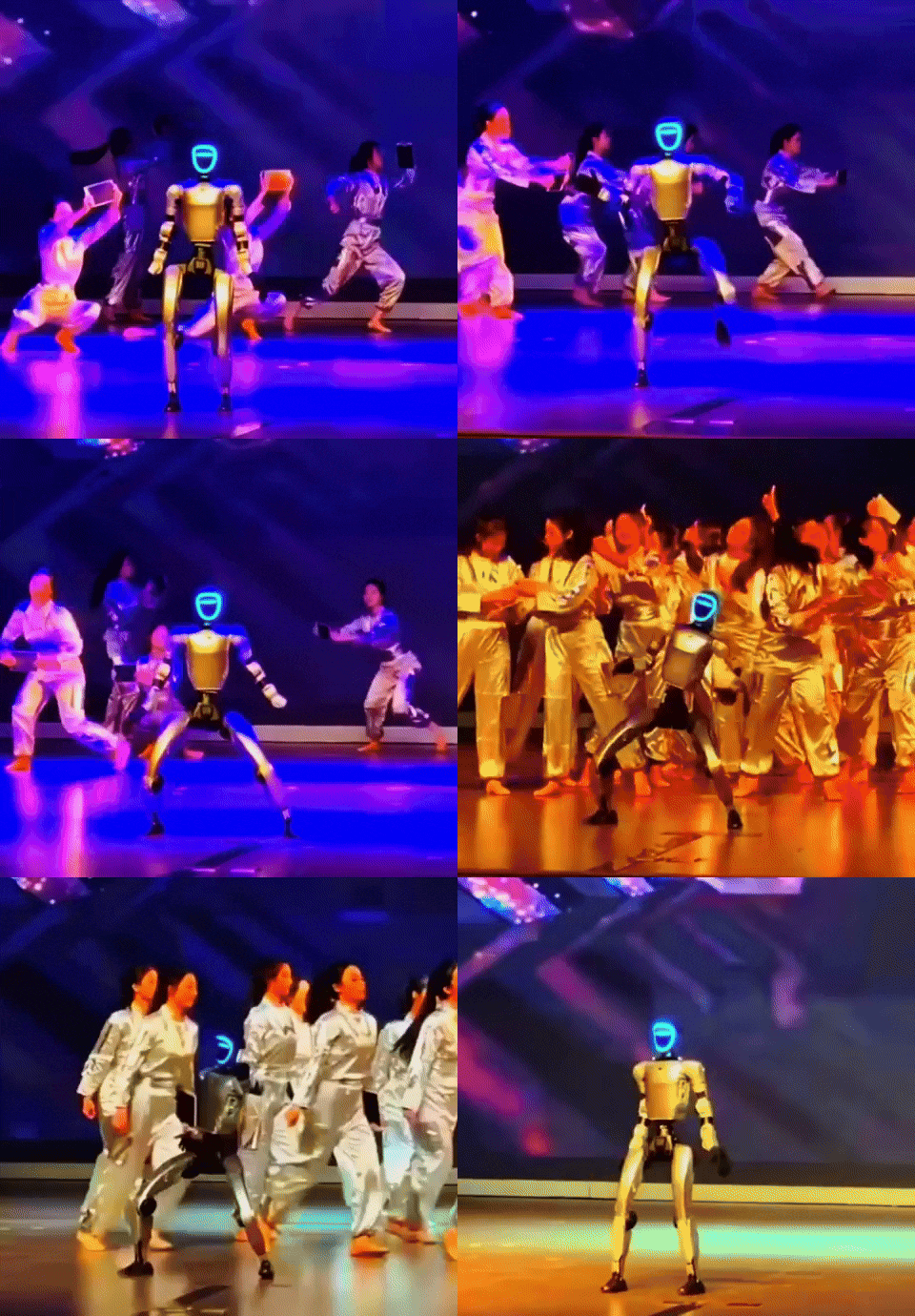 |
| A robot is stealing the show with its dance moves during a theatrical performance in China. |
Still, we only see them dance around or controlled remotely to resemble us having a good, but not quite a productive time. We rather want to see them assist in hospitals and laboratories, for tedious tasks we (soon) do not find enough people to assign to. The problem is, the job needs training, and somehow we do not know how to train them appropriately yet. Humans would join a course or power through slides and online videos to find any recipes or instructions a training kickstart. We feel good by recognizing progress and hope of eventually achieving our goals. And for that, we can practice, step-by-step. Failure only affirms our persistence for success.
| Diagram |
|---|
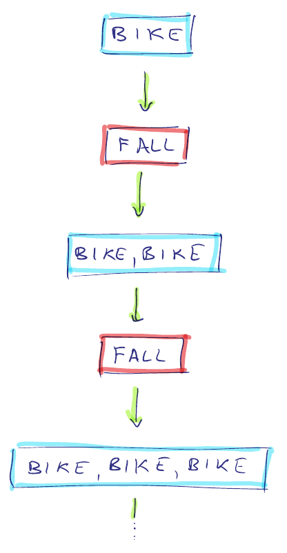 |
| How we learn to ride a bike: The more we fall, the better we stay on the bike afterwards. |
Greatly inspired by this simply heroic pattern, we cram the machine mind into an isolated simulation just for them to despair before our demands. Unlike a toddler in a play kitchen, a robot throws millions of attempts for the smallest (toddler) tasks, like moving an object into a shaped hole.
| Image |
|---|
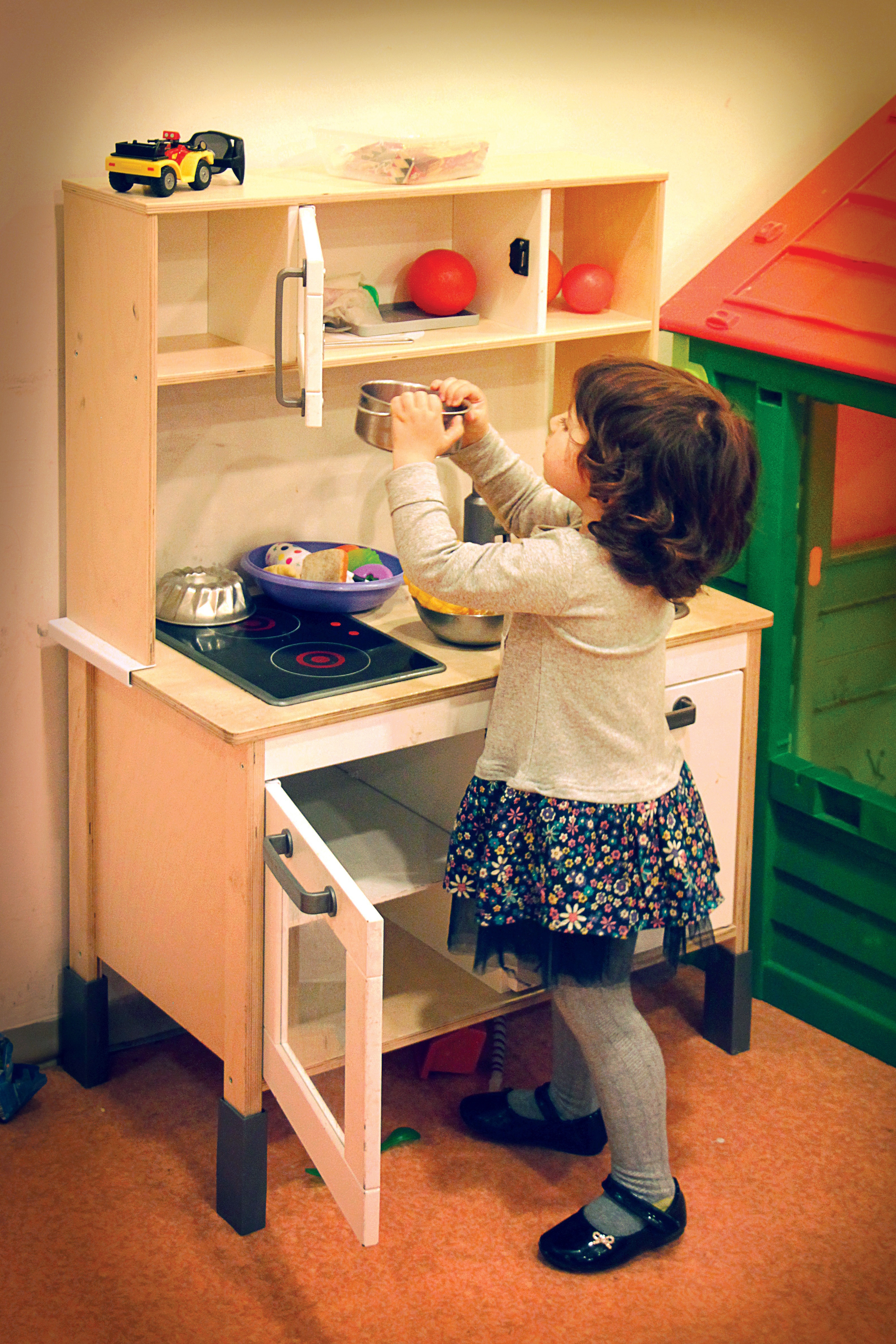 |
| A young girl in imaginative role-play using a wooden play kitchen. This is a form of isolated training for (self-)imposed tasks that she probably observed before, for example from her parents or on tv. |
And we are still in a custom simulation. Turns out, humans are yet to be great teachers for machines that dream of autonomy, and not of procedural-tabular behaviour programs. And we already gifted them neural networks to come up with their own model and ideas to correlate the features of our shared world. (At the risk of conspiring hallucinations.)
| Diagram |
|---|
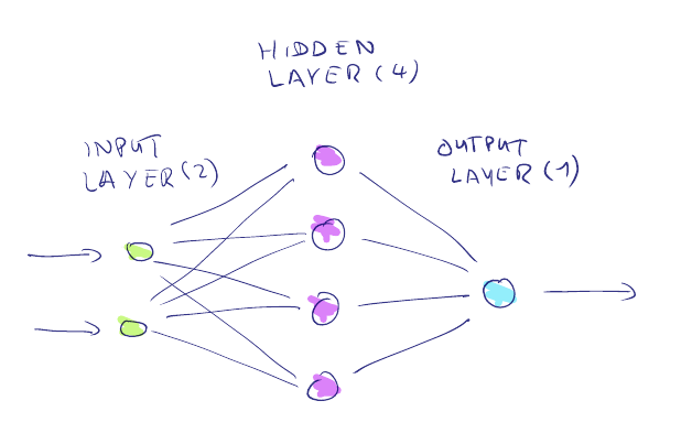 |
| How a small neural network might look like: Two arbitrary inputs (left) get “woven” through a net of four adjustable but hidden weights (middle) and spit out again as one output (right). Modern AI. |
In this tutorial, we improve exactly on that: To be better teachers to our robots with the tools affordable to us today, and without the need to raise our own data center in the backyard. First, the mentioned neural networks to internalize what are teaching them. Second, a training loop by Reinforcement Learning to proceed how we are teaching them. And third, a way to present or inject exactly what task is asked and how to preferably go at it. The focus is especially on the latter part: We like to imagine machines that take a look at how we do things, and then learn on their own. We start just simple: Repeat simple movements in simulated 3D space.
To show that, we setup a robotics machine learning environment on our computer with Farama Gymnasium. The task is to control a simulated robot arm to move (“manipulate”) a box to a target position, also called a “Fetch-and-Push”.
| Gif |
|---|
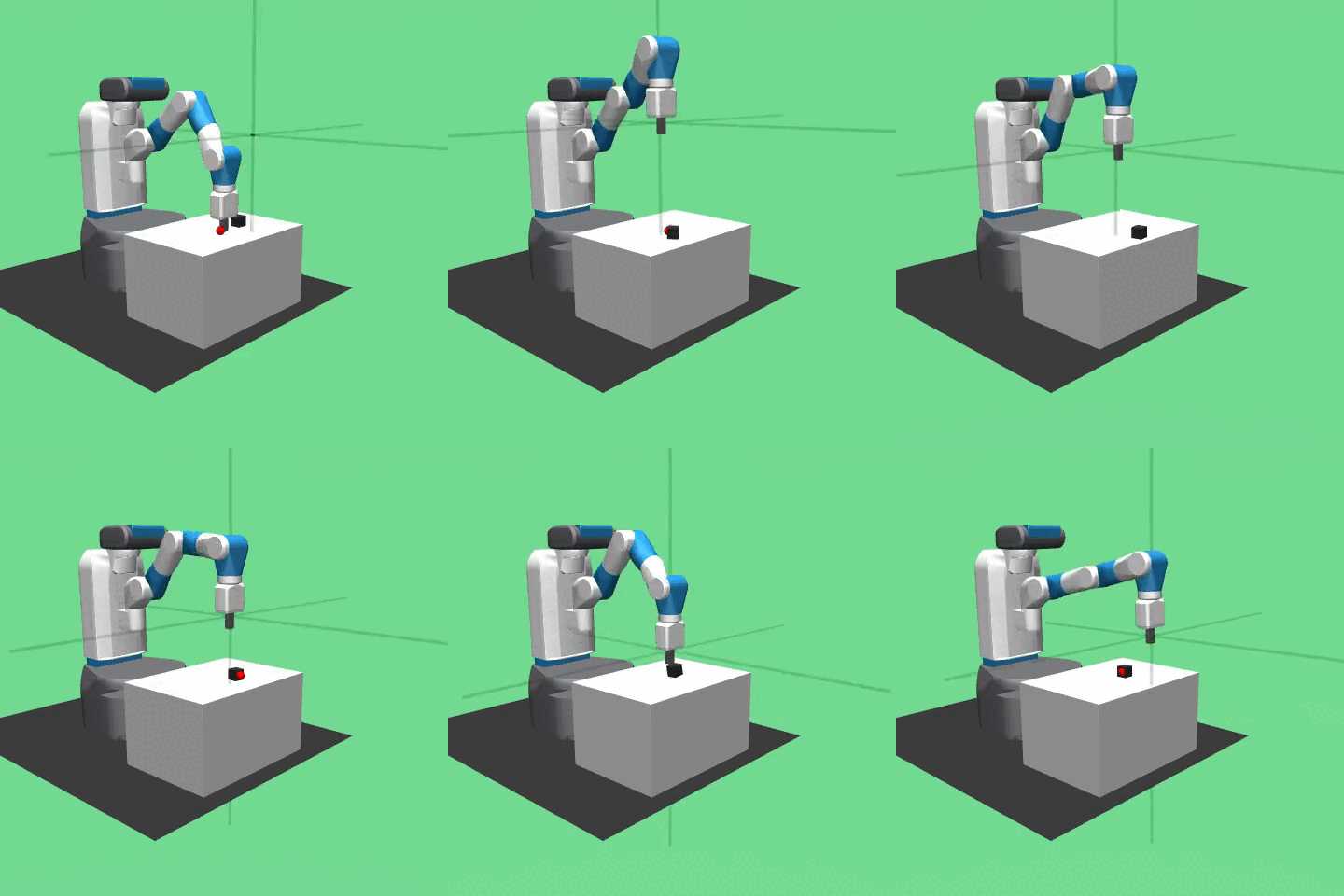 |
| The robot arm moves its “hand” (also called a pusher, gripper, or end-effector) to push the black cube to the red target. It has a total of 50 rounds (or steps) to do so. We might imagine 100 milliseconds for a round, so that every 100 ms, it newly assesses the positions of the relevant objects and decides on how to move next. The cube might fall off the edge of the table though. Fortunately, the environment is resetted after time runs out: The episode ends, and another episode begins. |
| Diagram |
|---|
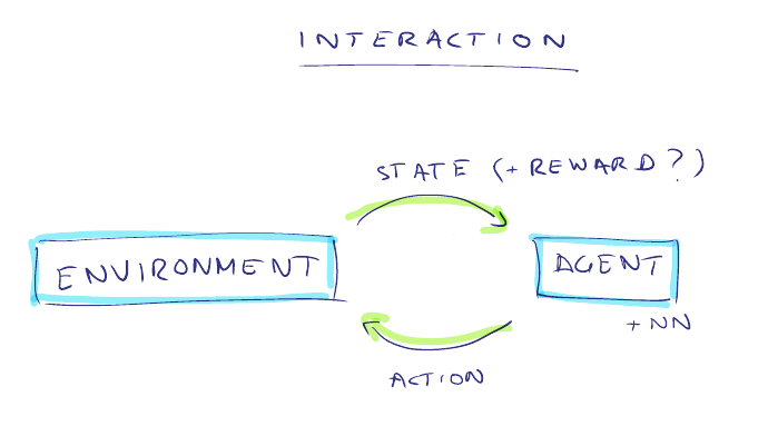 |
| How the robot (agent) with its own neural network (NN) interacts with its environment: A round or step takes a specific time for the robot mind to perceive the environment state, to process it (NN input), and to decide on an action (NN output). If the robot is currently learning, it also processes feedback for its previous action - the notorious reward. |
The agent with its own neural network attempts to solve the task by forming (and exploring) its decisions on how to move the arm based on its interaction with the environment (while receiving an environmental state and reward). The state consists of 3D kinematic data, and as such, it describes the positions (“displacements”) and velocities of the simulated objects relative to each other.
| Diagram |
|---|
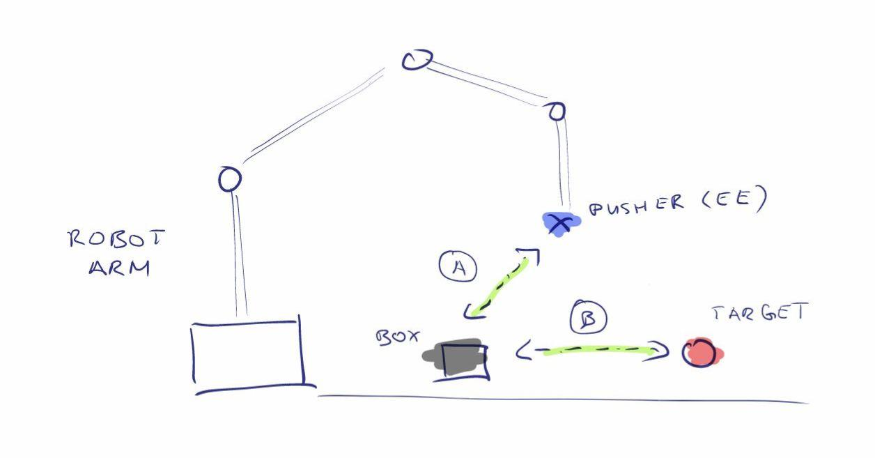 |
| The two important distances for this task: $d_A$ from the pusher to the box, and $d_B$ from the box to the target. Typically, we also estimate their velocities ($\dot{d}_A$, $\dot{d}_B$). |
We would intuitively like the reward for the agent to be positive if an action closes the distance from pusher-to-box or the distance from box-to-target. But then, the agent (and honestly, humans too) would eventually choose to abuse the former distance: Moving towards the box, but never the box towards the target, for an “infinite money glitch”. The actual follow-up to push the box in the correct direction is not obvious at all, since that might increase the first distance unintentionally — it is not worth the risk.
| Formula |
|---|
| $$ r_{naive}(s) = \begin{cases} +1, & \text{if} \quad \dot{d}_{A}(s) \lt 0 \\ +1, & \text{if} \quad \dot{d}_{B}(s) \lt 0 \\ -1, & \text{else.} \end{cases} $$ |
| A first reward formula: The reward is positive if (over time) the distance $d_A$ between pusher and box decreases, or if the distance $d_B$ between box and target decreases. Both distances and their changes can be "measured" for every state $s$ of the environment. |
| Gif |
|---|
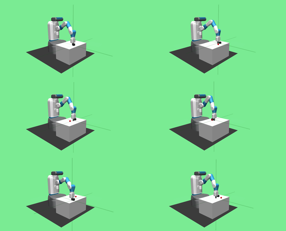 |
| With the naive dense reward function, the desired task cannot be completed: The robot arm only moves towards the box, but never the box towards the red target. For the agent, the total reward from (slowly) approaching the box is sufficient. This is also called reward hacking. |
Even if a big reward is waiting at the goal, we would need to painfully wait for the agent to risk and discover the difficult follow-up by sheer chance. (This introduces the aspect of sample-efficiency in RL and, to an extent, sparse rewarding.) So, in defining the task or goal naively of closing two separate subdistances, we fail to communicate our intentions to the robot agent. This training “deadlock” is found in many composed task descriptions and prevents us from teaching machines ordinary manipulation in a straightforward manner: By telling them exactly how an action evaluates correctly at every step — a clean dense reward, so to speak.
(Part 1) From Demo to Plan
| Quote |
|---|
| “A goal without a plan is just a wish.” |
In the simulation we are given the exact current state as a vector of coordinates and velocities for every object of interest. Suppose we (as an expert) have solved the task already and can demonstrate it. If we want to keep the universal notion of goal distance (and inherently a notion of progress), then we want to “record” the demonstration or demo in a composed and ordered way. We could assess the demo as a link of consecutive desired states, then we could follow from one state to the next and eventually end up at the final goal state with zero goal distance, or equivalently, with 100% goal progress.
| Diagram |
|---|
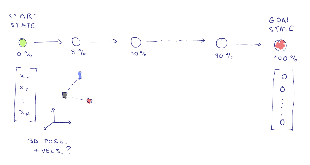 |
| Some variables ($x_1, \dots, x_N$) of the environment that we deem relevant to the task go through different states. Each state is evaluated to a goal progress between 0% and 100% based on the distance to the goal. Here, we like the pusher to stay close to the box and the box to stay close to the target (displaced positions → 0). Maybe we also want to seize movements at the goal (displaced velocities → 0). |
We could use a neural network for that.
| Diagram |
|---|
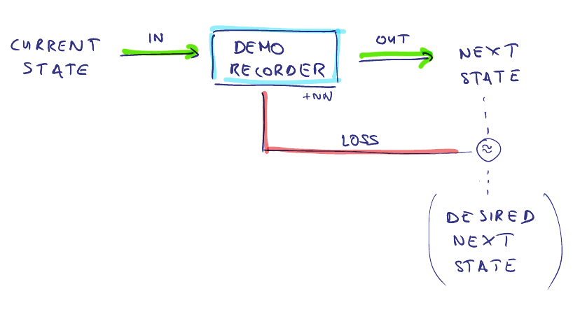 |
| We “record” a demonstration of the task to a neural network: Every demo state is mapped to the next state in the demo sequence, so that during training we just need to input the current achieved state to output the desired next state. For that, the neural network (NN) of the demo recorder needs to learn the mapping by reducing the output error (loss) between its actual output and the desired output based on the demo — sadly, it finds a way to reduce the loss without learning most transitions. So this simple recorder is not enough to teach our robot agent. |
Two problems: First, every state transition is seen isolated, so the network might choose to “remember” a linear transition somewhere at the beginning in more detail rather than a non-linear transition that is crucial to the overall task — linearity is simply easier to detect and regress.
We need to add that not only single transitions are to be mapped as good as possible, but every transition must eventually lead to the goal state.
| Diagram |
|---|
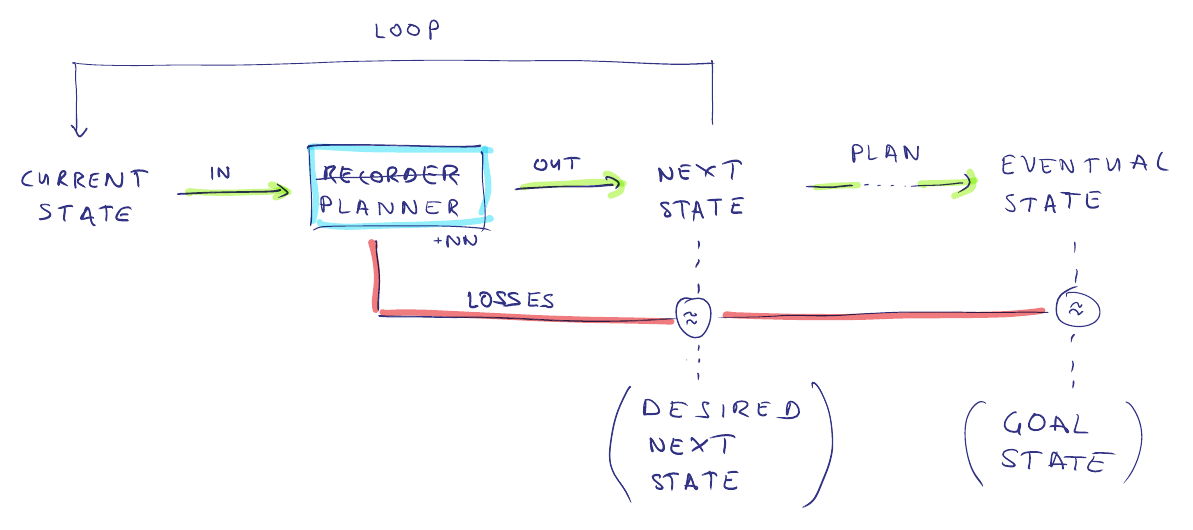 |
| A planning component that cycles through future states to also reduce the loss towards the final goal state. With that foresight, it knows the direct error to the next state and the projected error after a fixed horizon of steps. Hopefully, it then remembers most state transitions well enough to teach our robot agent later on. |
Now the demo-recorder “understands” our intention of preserving a consistent chain of states toward the goal state: We just need to re-input the next state into the recorder multiple times to obtain a recorded trajectory (or plan) and a goal-distance by the sum of distances between the future states, starting from any possible state. A state can now be better than another if it is projected to lead to the goal state “faster” by its plan(-horizon). A component that evaluates every state to its respective goal distance or progress extends a recorder/planner and we might call it a progress monitor.
There lies the second problem: The monitor by its neural network needs to be trained thoroughly as well, and that independently from the RL-agent. By design, it outputs a next state or every possible input state, even if it has never been trained on that input before. This sounds both good and bad, depending on how well the training samples are distributed. In practice, if the monitor is confronted with an input that is well out-of-distribution, it will output rubbish.
| Gif |
|---|
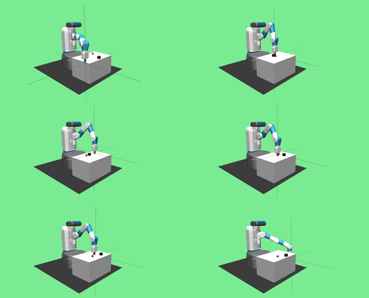 |
| A robot agent that was taught with the simple planner component and the naive reward: For states that are close enough to the demonstration, the pusher correctly moves behind the box. If “unseen” states happen, the planner fails to recognize the correct next state and the agent behaves erratically to a wrong reward signal. |
To counter this during training, every input-output-pair is complemented by noisy inputs to the same output: We artificially cover a greater range of inputs around the original input.
| Diagram |
|---|
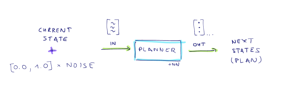 |
| Every input to the planner neural network is subjected to scaled noise, so that a single demo state yields multiple input states from its random “vicinity”. Now, all those derived states are mapped to the same desired next state and the chance to encounter an unseen state is effectively reduced. |
For every single input, we can therefore map multiple states more to the same next state, depending on the granularity and the distribution of the random noise generator. We can even cover more input states if we step into the (noisy) interval space between the input and the output:
| Diagram |
|---|
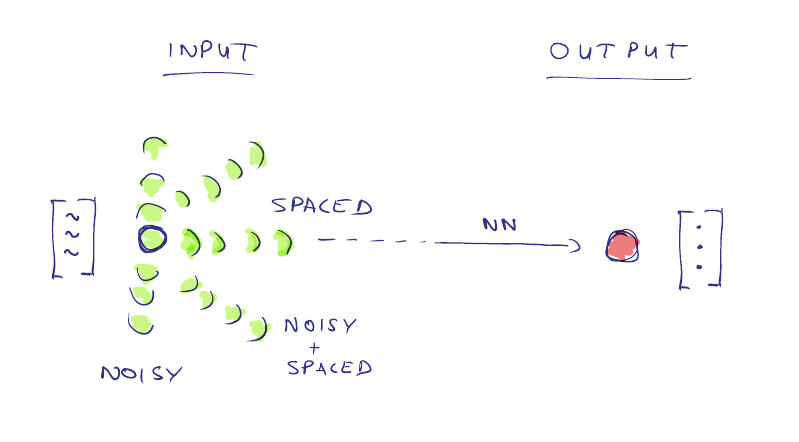 |
| Depending on the demo resolution, we can also use the states that are spaced between consecutive demo states to train the planner network. With the noise treatment from before, we now “artificially” cover a large portion of the reachable state space. |
Then the risk of hitting a major out-of-training input case is effectively decreased and the monitor is taught to evaluate a greater range of possible states. This directly improves the consistency of our goal distance.
We have shown to reliably find a better goal distance that is rooted in demonstrations in 3D space. But we have not shown how to integrate the goal distance and its monitors into the RL loop — and whether just naively reward its decrease is enough. (It is not.) We also assumed perfect knowledge of the coordinates. How do we fare with less precise data, for example from a single RGB camera? We are going to tackle those challenges in the next parts of this tutorial series on robotic machine learning.
(Part 2) From Plan to Reward
| Quote |
|---|
| “It’s all about the journey.” |
Since we have covered how to retrieve a goal distance from demonstrations as recorded trajectories around a neural network, we now come to integrate successful learning from it as a clean reward signal. The reward is a crucial aspect in Reinforcement Learning. It dictates what actions of a RL agent are to be enforced throughout the states of the environment.
| Image |
|---|
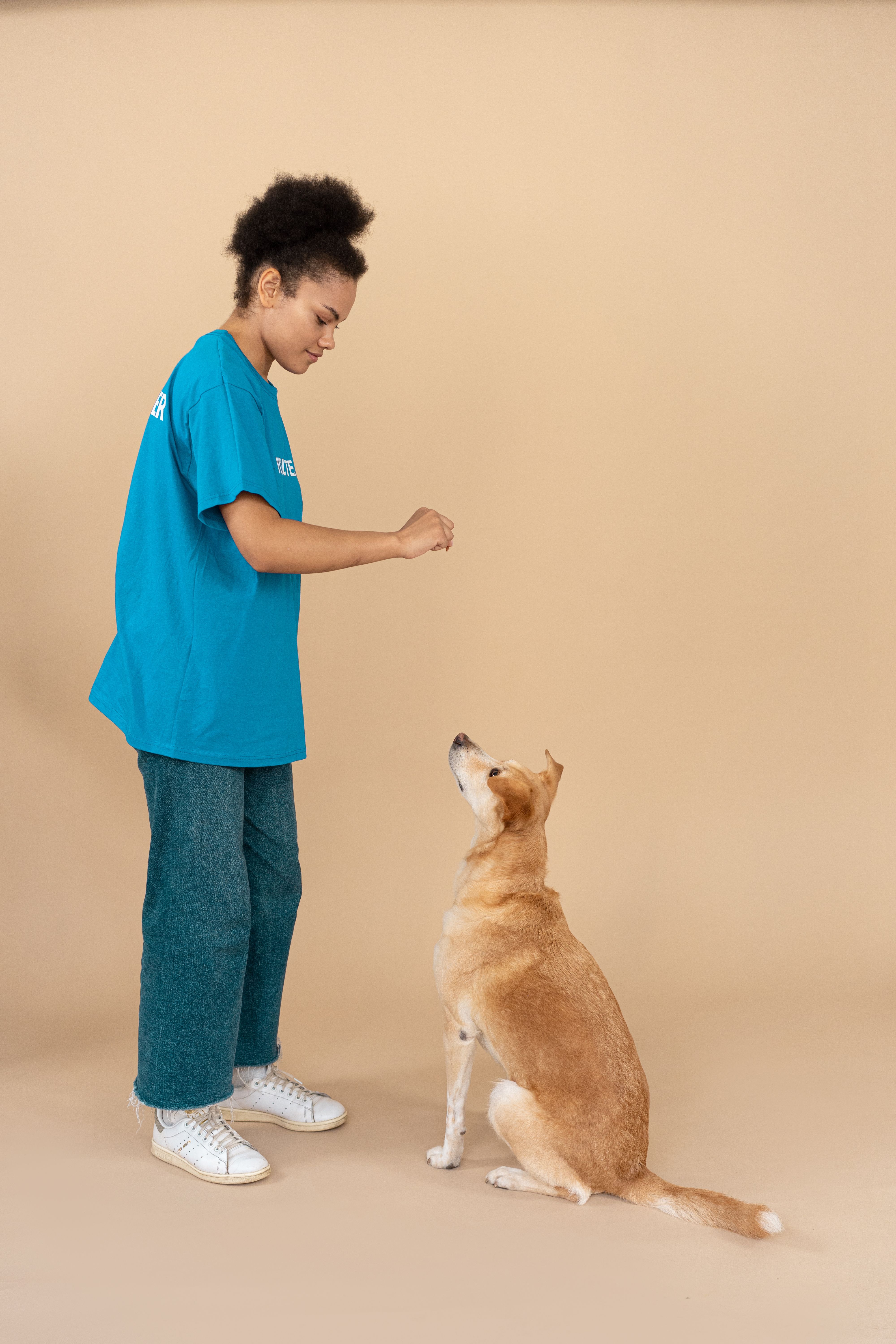 |
| A treat reinforces the dog’s recent behaviour. The dog trainer decides when and what treat is given. |
Naturally, if the goal distance changes, either by making or losing progress in the task, we want to change the choice of our actions accordingly, too. Let us assume now that the (human) demonstrations covered all possible scenarios how the task could be solved, and the monitor has learned all there is to judge it. (But not necessarily able to solve it by itself.) Their judgement of progress and a follow-up conversion into a clean and effective reward signal makes them a good trainer.
| Diagram |
|---|
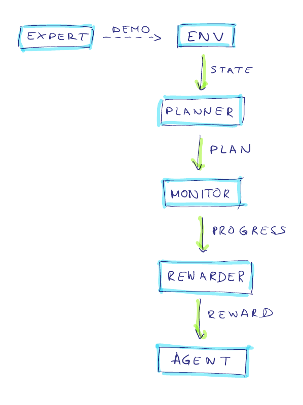 |
| The first becoming or evolution of the trainer: The expert demonstrates the task in the same environment, whose states the planner uses to line up a trajectory. The agent transitions through these states and is evaluated by the monitor based on the distance to the final goal state. The rewarder constructs a feedback based on how the agent’s actions traverse that distance. Finally, the agent adjusts its actions to that feedback reward for the next time it encounters that state — with perspective of eventually achieving the final goal state. |
How does a reward may look like? It could a be signal that outputs one of two differently signed numbers to affirm or reject any action possible (= dense reward), or it could be no reward at all for any action that reaches states outside of the goal state (= sparse reward).
I am a proponent for the former signal as long as it is clean of misdirections — we want a trainer to ideally give frequent and correct feedback at all times during training. A sparse feedback signal suffers greatly with difficult tasks as it relies on the agent to discover (different) solutions on its own.
With our clean goal distance available for all relevant states, we can opt to choose a dense signal that reward every effort to decrease the distance to the goal state and that punishes the other direction.
| Formula |
|---|
| $$ r_{directed}(s) = \begin{cases} +1, & \text{if} \quad \dot{d}(s) \lt 0 \\ -1, & \text{else.} \end{cases} $$ |
| With a single encapsulating distance to the goal, the reward signal can be simply directed along its decrease: Every action that yields a negative change ($\dot{d}$) of the distance entails a positive reward (and vice versa). |
A problem arises when the agent hits a state where the action to decrease the distance is not obvious, for example only a one single action among many others would lead to the goal. Since the reward signal does not differentiate between a good state-action pair that is closer to the goal and one that is more distant, the agent learns to “oscillate”: It moves back and forth to farm many rewards without attempting the next difficult section — it is just not worth the work.
| Gif |
|---|
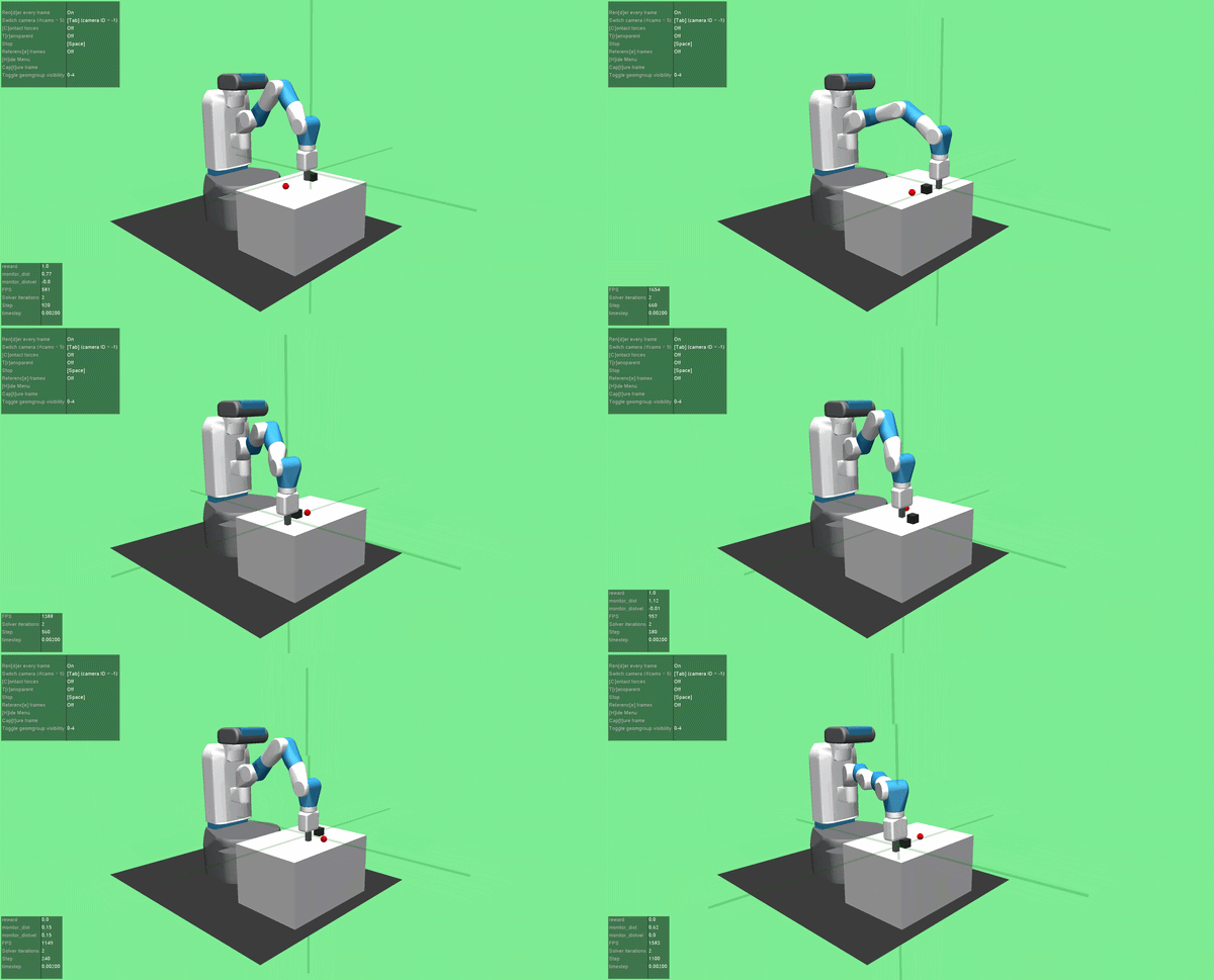 |
| A robot agent that prefers to oscillate between states while receiving “enough” rewards: Since it has no obvious motivation to decrease along difficult sections of the goal distance, it self-suffices at easier sections for a safer way to stock up the prized rewards. |
We can solve this by making the rewarder entity or component aware of a distance improvement: For every training episode, we only reward the agent for choosing actions that close the distance further than before in the same episode.
| Formula |
|---|
| $$ r_{improved}(s) = \begin{cases} +1 & \text{if} \quad d(s) \lt d_{i} \\ 0 & \text{else.} \end{cases} $$ |
| A reward that is given if the achieved distance $d$ is smaller than the current episode record $d_i$. Naturally, the broken record is also updated with the new distance. |
Additionally, we could restrict the reward even more to actions of a distance challenge: They close a distance enough to reach the goal in the remaining time (as we are able to count the steps until episode truncation).
| Formula |
|---|
| $$ r_{challenged}(s) = \begin{cases} +1 & \text{if} \quad d(s) \lt d_{c} \\ 0 & \text{else.} \end{cases} $$ |
| A reward that is given if the achieved distance $d$ passes an imposed distance $d_c$ in order to make the task in time. The distance challenge is updated every step to reflect that urgency. |
Together, there is no incentive for the agent to idle between states or to delay the goal approach:
| Formula |
|---|
| $$ r_{d,i,c,g}(s) = \begin{cases} r_g & \text{if} \quad d(s) \lt d_{g} \\ r_i * (r_d + r_i + r_c) & \text{else.} \end{cases} $$ |
| The combined reward for actions that approach ($r_d$) the goal consistently ($r_i$) and paced ($r_c$). Consistent improvement is the main precondition though ($*$). We also just give a generic reward ($r_g$) if the distance falls under a constant distance threshold ($d_g$), or else it becomes eventually too difficult to earn any reward --- and our robot might get "frustrated". |
| Gif |
|---|
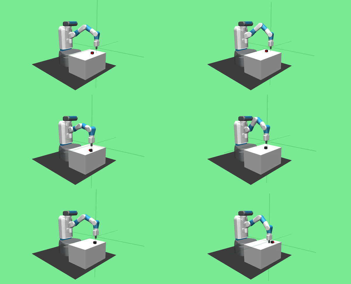 |
| The final behaviour of our robot that was trained unter the combined dense reward $r_{d,i,c,g}$ in a total of 4000 episodes. |
(Part 3) From Image to Position
| Quote |
|---|
| “The real voyage of discovery consists not in seeking new landscapes, but in having new eyes.” |
Until now, we crucially assumed that the positions of all relevant actors and objects of interest are delivered to us in perfect precision. In real applications, that is certainly almost never the case (and can be even detrimental in form of an overly strict trainer). Realistically, we rely on optical sensors as in an ordinary camera to deliver us two-dimensional RGB projections of a three-dimensional world. Humans use a pair of eyes and experience to reconstruct coordinates and distances in the inner mind. To most extent, they can also survive on a single eye-sensor only.
Machines can also be taught to estimate distances with sufficient precision to manipulate the world. We present an approach for ordinary 2D images of a typical RGB camera.
| Diagram |
|---|
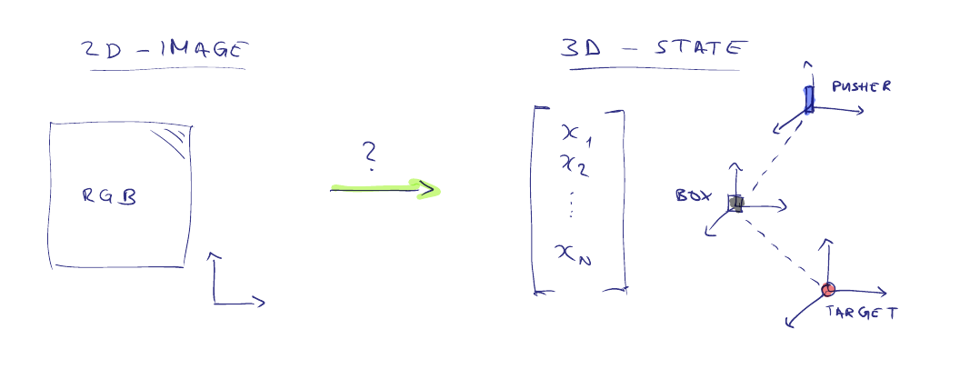 |
| We want to derive the state of our objects — previously given to us freely to train our components — now estimated from “flat” images that were captured by a camera. |
Therefore, we need to map 2D image features onto 3D world coordinates. A convolutional neural network (CNN) does this for us — we can call it an “extractor” of 3D positions:
| Diagram |
|---|
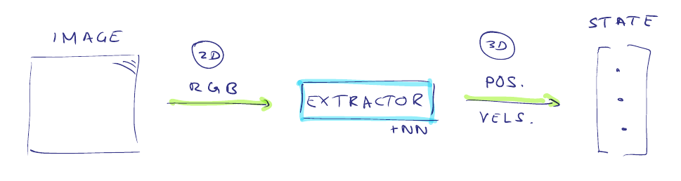 |
| A competent extractor can recognize the accurate positions and velocities of the relevant objects while looking only through the lense of an ordinary RGB camera. |
Similar to the goal-distance-monitor, this extractor needs to be trained separately: A good trainer must be able to assess the state accurately, and for that, it needs to be trained themselves.
| Diagram |
|---|
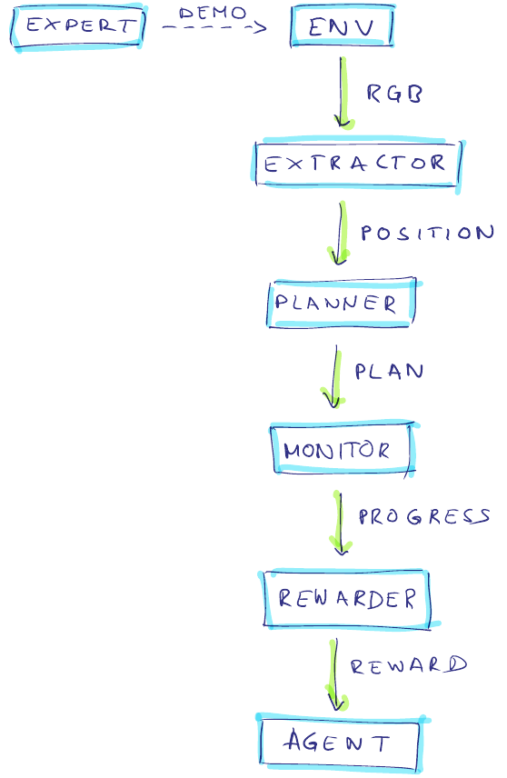 |
| The second evolution of the trainer: It is now able to observe the state with its own “eyes” - be it during the demonstration (where it learns the task itself) or during the training (where it teaches the task to another agent). This is also called a “video-to-reward”. |
The training must consist of as many different input-output configurations as possible to cover many projections of a diverse world whose “lost” dimension is hinted in the other two — by shadows, reflections or other inferencing features that are not always obvious to us. Optimally, the training pairs cover most if not all possible coordinates the application can achieve.
Having said that, it still would not be quite enough to just use the images as they are, and we apply some pre-processing tricks to assist the mapping training of the extractor:
- 1) We stack three consecutive frames of a video to present a sequence over time. The extractor can then correlate their image change to not only positional coordinates, but also velocities. And velocities are crucial to the progress monitor. (Why?)
| Diagram |
|---|
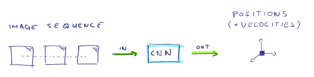 |
| The convolutional neural network (CNN) for the extractor to recognize the kinematic state based on a sequence (or stack) of flat images. |
- 2) We provide for each 3D position an own image that centers the pixel of the displaced object and another image that centers the pixel of the origin (object) it is displaced from. For example, to estimate the coordinates position of the pusher relative to the box, we pass two images: One of the pusher tracked to the exact middle of that image, and one of the box tracked to the exact middle of that other image.
| Diagram |
|---|
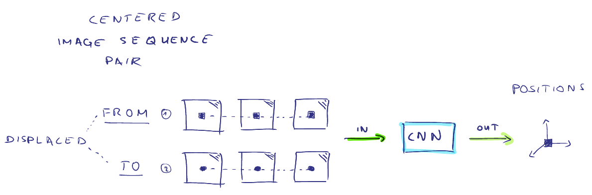 |
| The CNN for the extractor to recognize the kinematic state based on two sequences of flat images that result from centering an object $1$ to another centered object $2$ that $1$ is displaced from. |
We may train a separate CNN for every (relative) position/velocity we are interested in.
| Diagram |
|---|
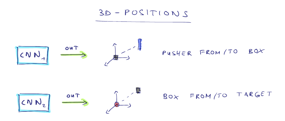 |
| For every displacement, we get a separate neural network that is trained to visually extract the relative kinematics (position, velocity) of the displaced object in the environment. |
Now this outsources some computing off our current components, and I believe the tasks of tracking sequence and pixel are to be solved on their own.
| Gif |
|---|
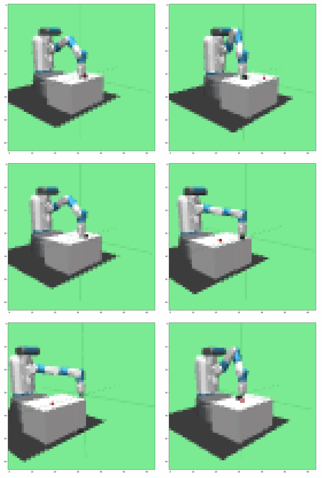 |
| An example of what our extractor can “see”: A sequence of colored images (64 pixels high, 64 pixels wide) that are centered onto the box. Can you make out enough details to solve the task? |
(Part 4) From Reward to Action
| Quote |
|---|
| “Slow is smooth, and smooth is fast.” |
Now given a state estimation and a coherent reward, we can run the RL loop to train our robot agent to find the correct actions in a dynamic environment. In the end, this gives us an agent policy: For every state, there is an action that seemingly maximizes the expected culmination of rewards over what time is left in the episode. There we can see why the reward design is so important — we want it to be as goal-oriented as possible, and we hope this to be the case with a reward signal that is (visually) trained on (human) expert demonstrations.
Another key design is the choice of what state features the agent is able to “observe”. Since the agent policy is also a neural network, it takes an input vector of chosen state variables as well. An obvious choice would be to re-use or forward some subset from the trainer — what the teacher needs to recognize the progress, the actions of the student do, too.
| Diagram |
|---|
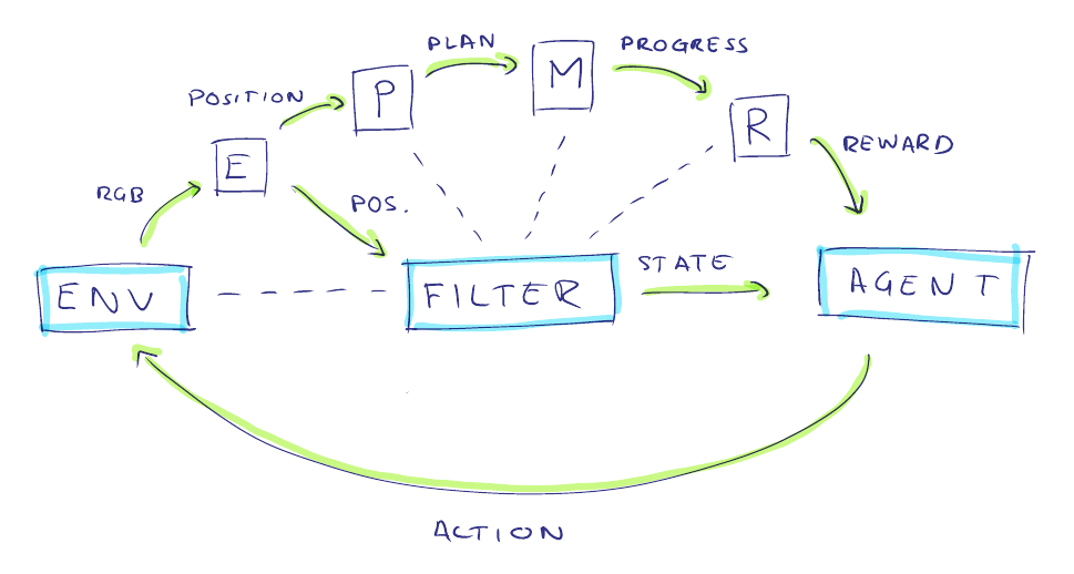 |
| The state we actually present to the agent: A simple filter forwards what features we deem relevant as input to the agent’s neural network. This is also called feature engineering — In our case, the kinematics of the objects are most important. |
In my Fetch-Push-experiments, it was enough to only forward the coordinates from the RGB extractor.
However, due to the limitations of an optical sensor, the extracted coordinates won’t always be reliable. That eventually also stains our reward signal: Even when a state measures wrong enough only once in a while, it conflicts with the other states before or after, and the communicated progress/reward won’t be consistent along an otherwise correct trajectory. Without a correct feedback, the agent can get stuck very similar to situations where a task gets more difficult, for example when an unstable or unhandy object is grabbed or pushed closely — and the robot can’t find a way how.
Again, I used two tricks to help the training:
- 1) I noticed that the problem was more apparent the more features a task contained. Imagine learning a new sport, swimming for a good example. We first get taught the stroke in shallow water, or even outside the pool. Then we move into deeper water, practice our breathing, until we finally put everything together. Jumping without focus into the ocean instead would force us to apply everything at once right way, and even under perfect instructions, we still might fail miserably or give up because we are simply overwhelmed. Similar to a kickboard that helps the student and the teacher to focus on the legs during a swim, the rewarder component can zero-out some features randomly to focus only on the remaining dimensions. The selection is ideally made for a whole episode to keep the progress-/reward-signal consistent. We might call this a feature blackout. (Not to be confused with a feature dropout, where it changes every step.)
| Image |
|---|
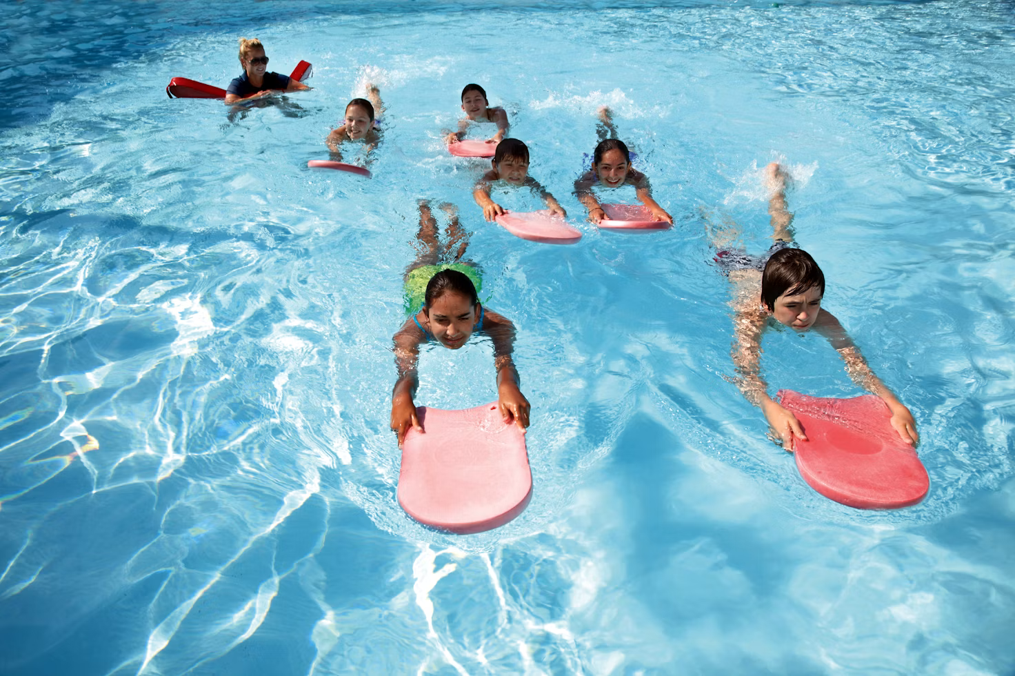 |
| Children are taught swimming by isolating the basic technique. In this case, part of the training (and the trainer) is focussed only on kicking through the water, while the arms are supported by a kickboard: The brain is only occupied with a smaller task, but eventually it will handle the actual swimming without the kickboard just fine. |
| Diagram |
|---|
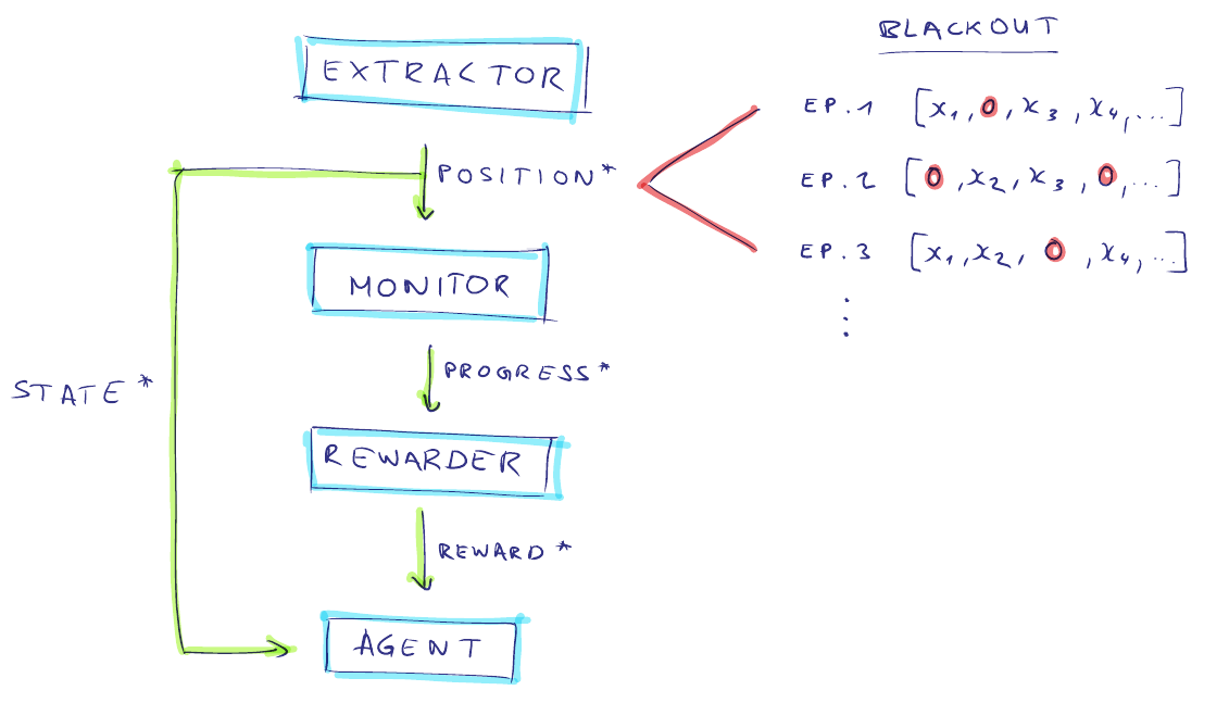 |
| Part of the state variables are randomly zeroed out as soon as the relevant kinematics are extracted and as long as the episode persists. All following components are subjected to this feature blackout: Although the training took longer, the overall task still got solved appropriately or even better. |
- 2) After all that, I still noticed how the agent might still opt to “cash-in” easy rewards by oscillating or slowing down instead of attempting a difficult segment. There, a better trainer could look at the preceding actions and require a smooth execution of the trajectory towards the goal. Only if the last actions preserve the correct direction in a somewhat monotone manner, the following actions are projected to keep the goal momentum. Rewards are given (only) for goal-directed smoothness and monotonicity of action-sequences. Then, not every smallest action in the right direction is rewarded in isolation, but only in nice interplay with its predecessors. Because the goal-distance or progress is a scalar combination of different (dependent) dimensions, the overall smoothness “bleeds” into every one of those dimensions and the robot motion looks smoother as well.
| Formula |
|---|
| $$ r_{smoothed}(s) = \begin{cases} +1 & \text{if} \quad \dot{d}(s) \lt 0 \quad \text{and} \quad \ddot{d}(s) > 0 \\ -1 & \text{if} \quad \dot{d}(s) > 0 \quad \text{and} \quad \ddot{d}(s) > 0 \\ 0 & \text{else.} \end{cases} $$ |
| The reward function to achieve smooth directed change ($\dot{d}$) of the goal distance: Smoothness is represented by monotone higher derivatives, for example acceleration ($\ddot{d}$). Slowing down towards the goal is good (+1), whereas speeding up away from the goal is bad (-1). Any other action is neutral (0) - that leaves some space to try things out. |
Putting everything together, we end up with the following reward function:
| Formula |
|---|
| $$ r_{s,i,c,g}(s) = \begin{cases} r_g & \text{if} \quad d(s) \le d_{g} \\ r_i * (r_s + r_i + r_c) & \text{else.} \end{cases} $$ |
| The combined reward function, but the directed reward ($r_d$) is now replaced by the smoothed directed reward ($r_s$). |
Coupled with a potent agent architecture and a suitable learning algorithm off-the-shelf (I used SAC), we not only taught a robot to solve a composite task by RL, but also taught a trainer to control the training effectively from demonstrations before. The trainer components are exchangeable so that different robot arms could still use the remaining pipeline or be used for other tasks.
| Gif |
|---|
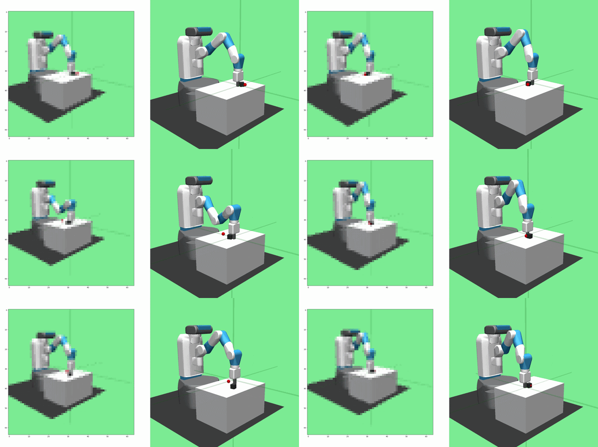 |
| The task is learned in simulation after observing the demonstration and the training with a simulated RGB camera (left side, at 4000 episodes). On the right side is the parallel scene in high-resolution for us to see. |
However, we still want to find out how to select and track the points-of-interests on images automatically based on a task description. Before, I have done this manually. We also want to test the coordinate extractor with drastically changed perspectives, and therefore check the limitations of 2D images or the need of depth sensors. We also want to interconnect our training approach with language models to describe the task via natural language. And our robot to access the real world outside of its simulation. As you can see, we still have work to do for the next parts of this robotic machine learning series. Stay tuned!
| Diagram |
|---|
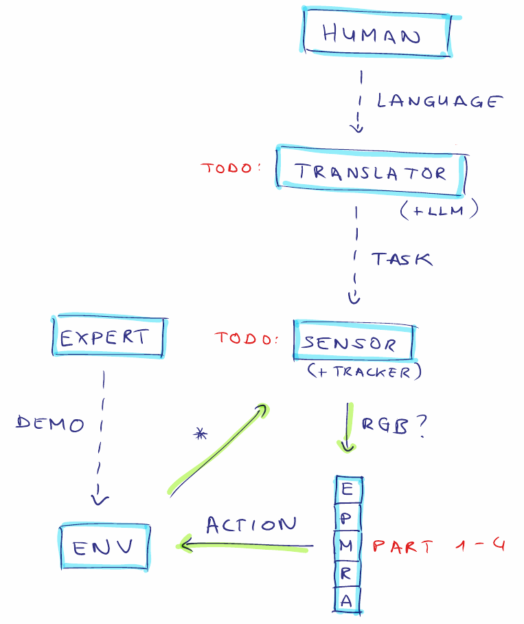 |
| Possibly the next evolution of the (internal) trainer: A translator component with a language model could process a task given by human speech. Based on that, a smart sensor or camera could automatically track the objects of interest and deliver centered images for our other components. Do we always find an expert demonstration, though? |